How To Set Up A Pivot Table - How To Create A Pivot Table How To Excel : Go to insert tab → tables command group → click pivottable create pivottable dialog box appears.. If you are using excel 2003 or earlier, click the data menu and select pivottable and pivotchart report. To create a blank pivot table: We can group our pivot table date by month, day. Select any of the cells from your pivot table. Click insert along the top navigation, and select the pivottable icon.
From this example, we are going to consider function in our filter, and let's check how it can be listed using slicers and varies as per our selection. You cannot use the merge cells check box under the alignment tab in a pivottable. Once you've entered data into your excel worksheet, and sorted it to your liking, highlight the cells you'd like to summarize in a pivot table. Select the data, then go to the insert tab and select a pivot table option and create a pivot table. But first, i needed to set up a formula that returns the number of rows in the pivot table.
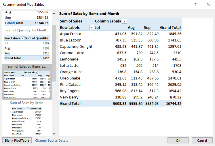
How To Create Pivot Table In Excel Beginners Tutorial from cdn.guru99.com Lastly, we will create our pivot table by selecting insert, then pivot table. On the analyze tab, in the calculations group, click fields, items, & sets, and then click calculated field. Start the pivot table wizard. Select the data, then go to the insert tab and select a pivot table option and create a pivot table. After that, we will assign date and products to the rows label as well as the sales to the values section; Click the pivottable button on the left side of the insert ribbon. I changed the pivot table's name to sales. Go to insert tab → charts → pivot chart and select the chart which you want to use.
While creating a pivot table, make sure there will be no blank column or row.
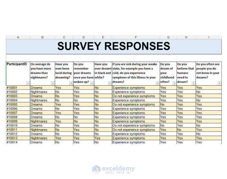
This is the source data you will use when creating a pivot table. This will greatly reduce the size of your pivot table. This action will prompt another window, which will show you some options about where you would like to place your pivot table. The first step to creating a pivot table is setting up your data in the correct table structure or format. Select any cell within the data set. While creating a pivot table, make sure there will be no blank column or row. Choose where to place your pivot table after clicking that pivot table button, you'll be met with a popup that asks where you'd like to place your pivot table. In the create pivottable dialog box, under choose the data that you want to analyze, click use an external data source. On the connections tab, in the show box, keep all connections selected, or pick the connection category that has the data source you want to. In the pivot table, always add the unique value in your column fields. On the analyze tab, in the calculations group, click fields, items, & sets, and then click calculated field. Now the pivot table is ready. We can group our pivot table date by month, day.
Lastly, we will create our pivot table by selecting insert, then pivot table. Once you've played around with the pivot table feature and gained some understanding of how the various options affect your data, then you can start creating a pivot table from scratch. In the pivottable options dialog box, click the layout & format tab, and then under layout, select or clear the merge and center cells with labels check box. In the pivot table, always add the unique value in your column fields. Creating a simple pivot table.
How To Create Pivot Tables That Provide Meaningful Data Analysis Insights from www.exceldemy.com After that, we will assign date and products to the rows label as well as the sales to the values section; Select any cell within the data set. Watch this short video to see the steps for creating a pivot table, after the data has been prepred. On the connections tab, in the show box, keep all connections selected, or pick the connection category that has the data source you want to. This tutorial has a quick overview of creating a pivot table. To set top 1 filter, simply click on the filter. Go to insert tab → tables command group → click pivottable create pivottable dialog box appears. We can group our pivot table date by month, day.
The first step to creating a pivot table is setting up your data in the correct table structure or format.
Click any cell on the worksheet. To do so, highlight your entire data set (including the column headers), click insert on the ribbon, and then click the pivot table button. To set top 1 filter, simply click on the filter. We can group our pivot table date by month, day. Set up the pivot table's sales.numrows range. Change the table/range value to the required cell range where your data set is placed. In the pivottable options dialog box, click the layout & format tab, and then under layout, select or clear the merge and center cells with labels check box. You cannot use the merge cells check box under the alignment tab in a pivottable. Once you've entered data into your excel worksheet, and sorted it to your liking, highlight the cells you'd like to summarize in a pivot table. Your source data should be setup in a table layout similar to the table in the image below. The first step to creating a pivot table is setting up your data in the correct table structure or format. For the pivot table, data should be in the right and correct form. Make sure your data is in columns with headers.
To create a blank pivot table: I added the text shown in cell a1 in the figure below. In the name box, type a name for the field. Now the pivot table is ready. I changed the pivot table's name to sales.
The Procedure For Calculating A Percentage In A Pivot Table Excelchat from d295c5dn8dhwru.cloudfront.net From the insert tab, choose to insert a pivot table. select the pivot table fields such as salesperson to the rows and q1, q2, q3, q4 sales to the values. Now the pivot table is ready. But first, i needed to set up a formula that returns the number of rows in the pivot table. Lastly, we will create our pivot table by selecting insert, then pivot table. If you already have a pivot table in your worksheet then you can insert a pivot chart by using these simple steps. If you are using excel 2003 or earlier, click the data menu and select pivottable and pivotchart report. Go to the ribbon and select the insert tab. Select any of the cells from your pivot table.
The following is a list of components of a data table.
I added the text shown in cell a1 in the figure below. The following is a list of components of a data table. To insert a pivot table, execute the following steps. After that, we will assign date and products to the rows label as well as the sales to the values section; Creating a simple pivot table. Start the pivot table wizard. Now the pivot table is ready. How to insert and setting up pivot table in excel. Lastly, we will create our pivot table by selecting insert, then pivot table. From this example, we are going to consider function in our filter, and let's check how it can be listed using slicers and varies as per our selection. Select the cells you want to create a pivottable from. Once you've played around with the pivot table feature and gained some understanding of how the various options affect your data, then you can start creating a pivot table from scratch. Your data shouldn't have any empty rows or columns.